Clustering and integration workflow
Songqi Duan
duan@songqi.org Source:vignettes/clustering.Rmd
clustering.RmdThis article covers the core unsupervised-analysis stage in Shennong using the built-in PBMC examples. The workflow shows how to move from a preprocessed Seurat object to:
- single-sample clustering
- multi-sample Harmony integration
- optional rare-aware feature selection before PCA/integration
- pre/post integration embedding comparison
- cluster visualization on the integrated object
Downstream metrics, composition, and interpretation now have their own dedicated articles, but a few summary outputs remain here so the integration workflow is visible end to end.
To keep R CMD check deterministic, the analysis is only
evaluated when SHENNONG_RUN_VIGNETTES=true or during
pkgdown builds.
Shennong also ships bundled human and mouse GENCODE gene annotations,
so sn_filter_genes() can combine expression-threshold
filtering with annotation-based retention such as
gene_class = "coding" or exact gene_type
subsets.
Inspect bundled signatures
Shennong now ships a tree-structured signature catalog derived from
SignatuR and stored as package data. You can inspect the
available signature paths and retrieve a specific signature either by
short alias or by full tree path.
signature_catalog <- sn_list_signatures(species = "human")
head(signature_catalog[, c("path", "n_genes")], 6)
#> # A tibble: 6 × 2
#>   path                   n_genes
#>   <chr>                    <int>
#> 1 Blocklists/Pseudogenes   12600
#> 2 Blocklists/Non-coding     7783
#> 3 Programs/HeatShock          97
#> 4 Programs/cellCycle.G1S      42
#> 5 Programs/cellCycle.G2M      52
#> 6 Programs/IFN               107

mito_genes <- sn_get_signatures(
  species = "human",
  category = c("mito", "Compartments/Ribo")
)
length(mito_genes)
#> [1] 205
Data loaded for the workflow
knitr::kable(cell_summary, digits = 0)| dataset | cells | genes | clusters |
|---|---|---|---|
| pbmc1k | 1141 | 24986 | 11 |
| pbmc3k | 2671 | 19971 | NA |
| merged_unintegrated | 3812 | 25597 | 14 |
| merged_integrated | 3812 | 25597 | 11 |
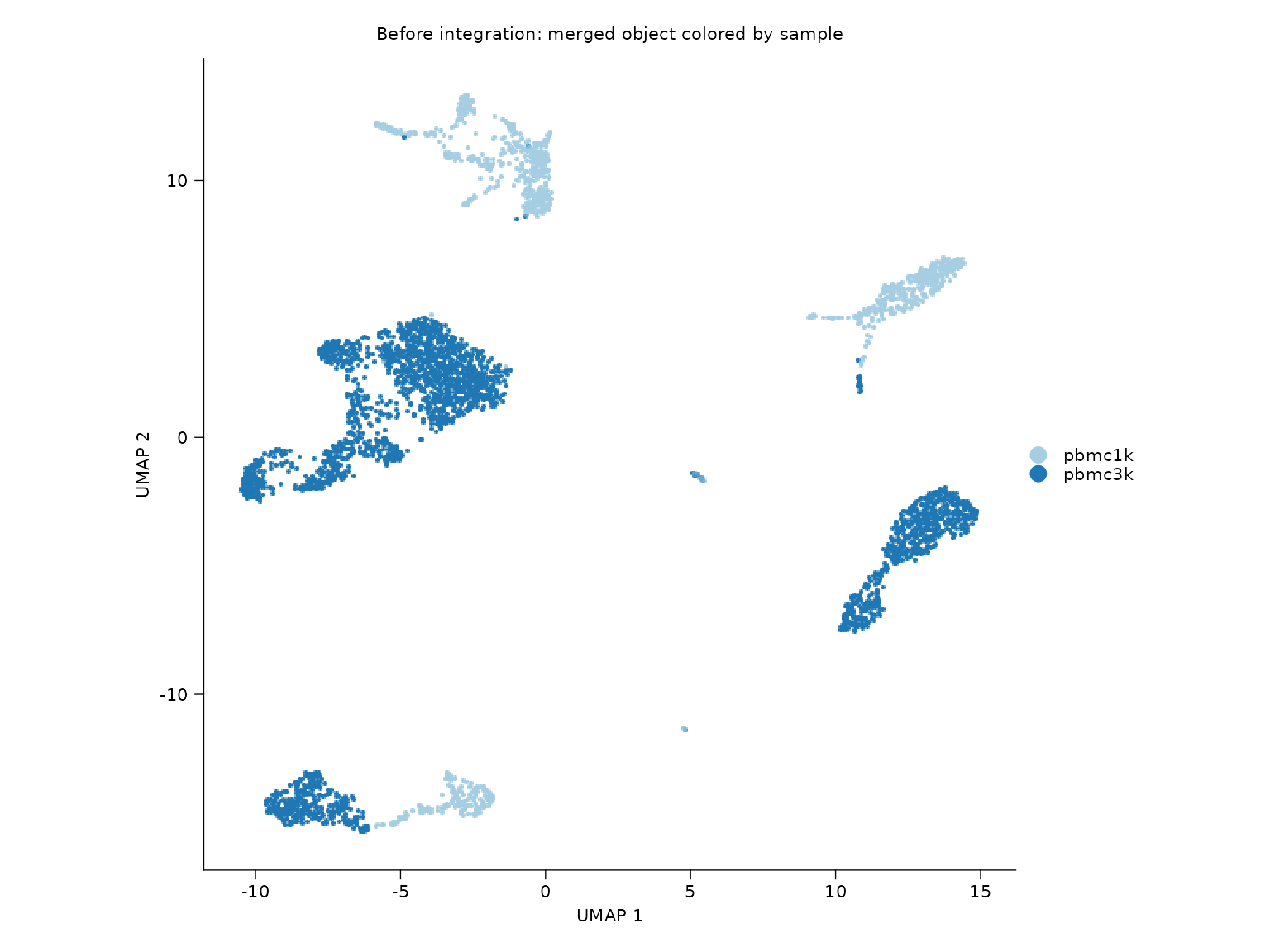
The merged analysis is intentionally run twice: once without batch correction and once with Harmony integration. This makes the before/after comparison explicit instead of only showing the corrected embedding.
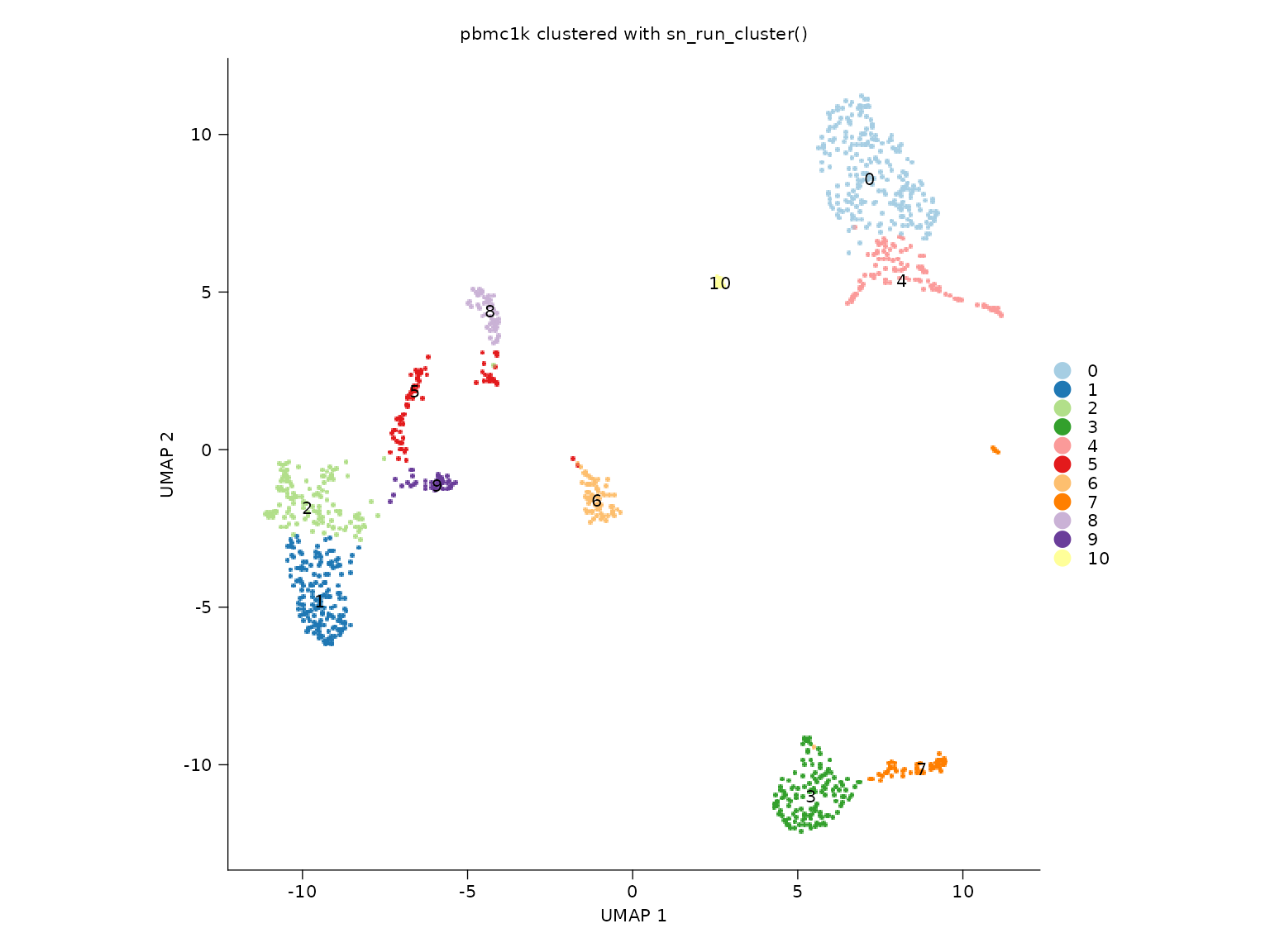
Single-sample clustering
sn_plot_dim(
  object = pbmc1k_clustered,
  reduction = "umap",
  group_by = "seurat_clusters",
  label = TRUE,
  show_legend = FALSE,
  title = "pbmc1k clustered with sn_run_cluster()"
)
Before and after Harmony integration
sn_plot_dim(
  object = pbmc_unintegrated,
  reduction = "umap",
  group_by = "sample",
  title = "Before integration: merged object colored by sample"
)
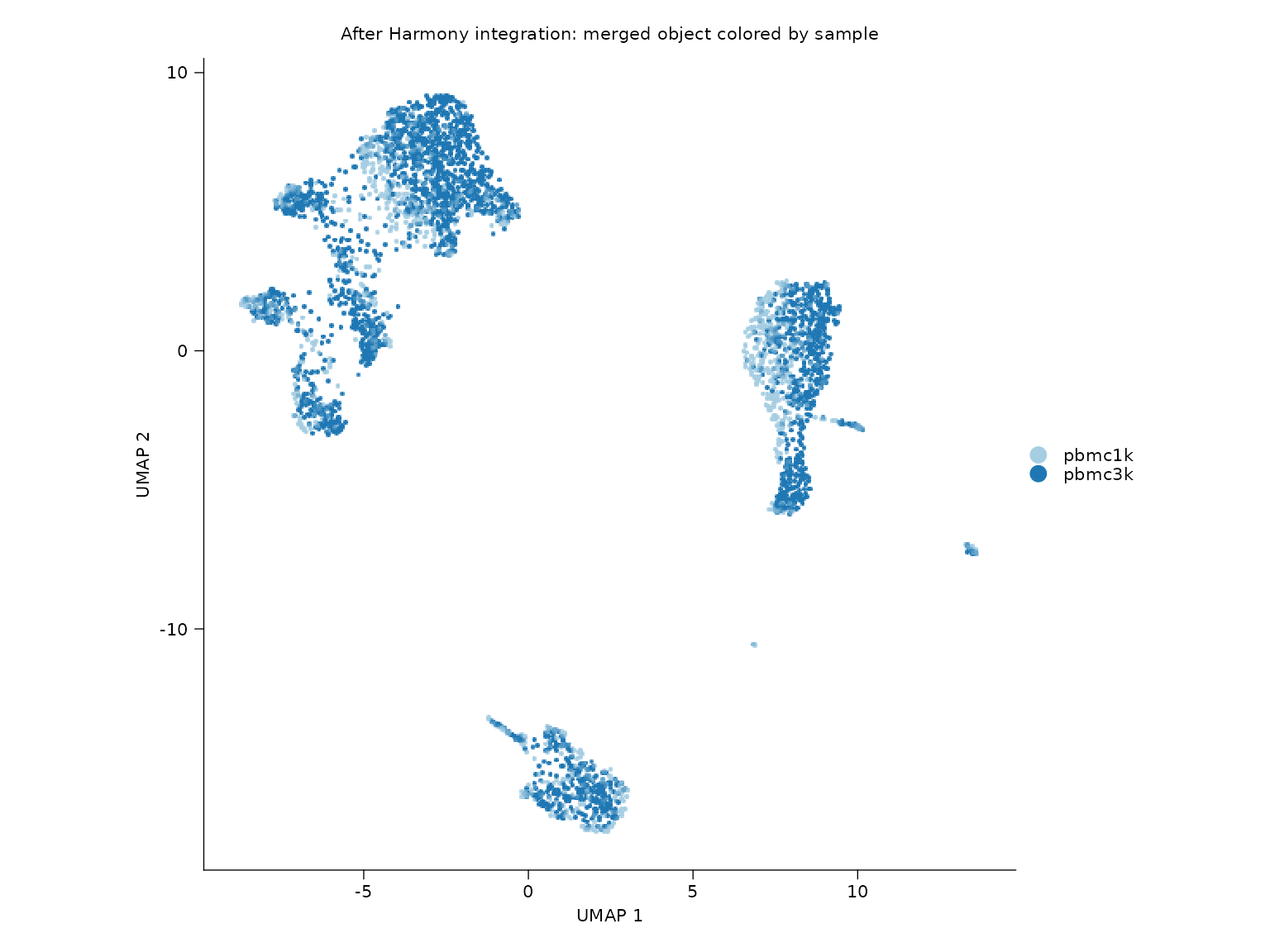
sn_plot_dim(
  object = pbmc_integrated,
  reduction = "umap",
  group_by = "sample",
  title = "After Harmony integration: merged object colored by sample"
)
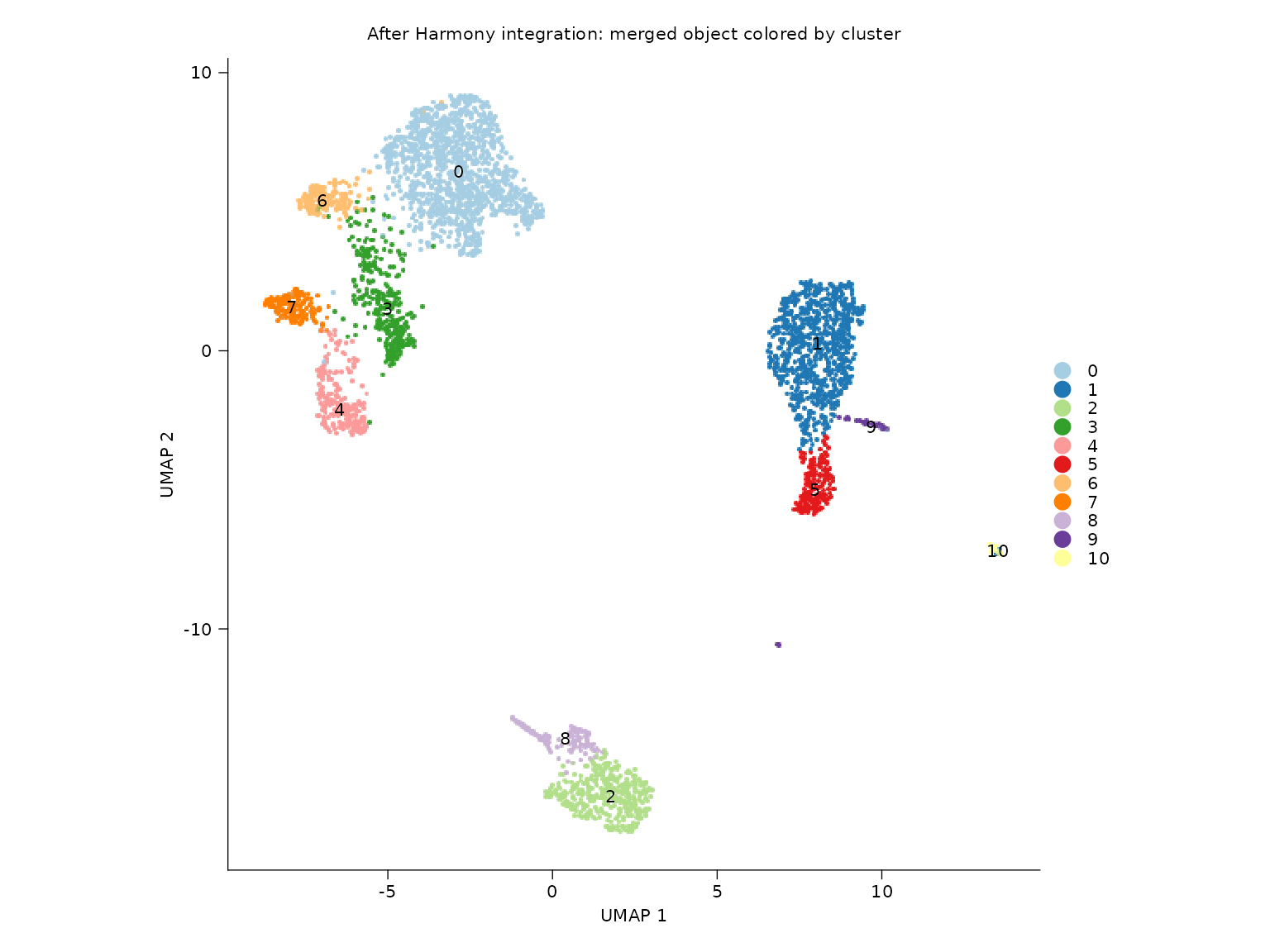
sn_plot_dim(
  object = pbmc_integrated,
  reduction = "umap",
  group_by = "seurat_clusters",
  label = TRUE,
  show_legend = FALSE,
  title = "After Harmony integration: merged object colored by cluster"
)
Cluster composition by sample
knitr::kable(dplyr::slice_head(composition_tbl, n = 12), digits = 2)| sample | seurat_clusters | proportion |
|---|---|---|
| pbmc1k | 0 | 27.61 |
| pbmc1k | 1 | 27.96 |
| pbmc1k | 10 | 1.31 |
| pbmc1k | 2 | 11.31 |
| pbmc1k | 3 | 5.96 |
| pbmc1k | 4 | 6.22 |
| pbmc1k | 5 | 2.28 |
| pbmc1k | 6 | 3.86 |
| pbmc1k | 7 | 6.13 |
| pbmc1k | 8 | 5.17 |
| pbmc1k | 9 | 2.19 |
| pbmc3k | 0 | 36.62 |
sn_plot_barplot(
  composition_tbl,
  x = sample,
  y = proportion,
  fill = seurat_clusters
) +
  labs(
    title = "Cluster composition across pbmc1k and pbmc3k",
    x = NULL,
    y = "Cells (%)",
    fill = "Cluster"
  ) +
  theme_minimal(base_size = 12)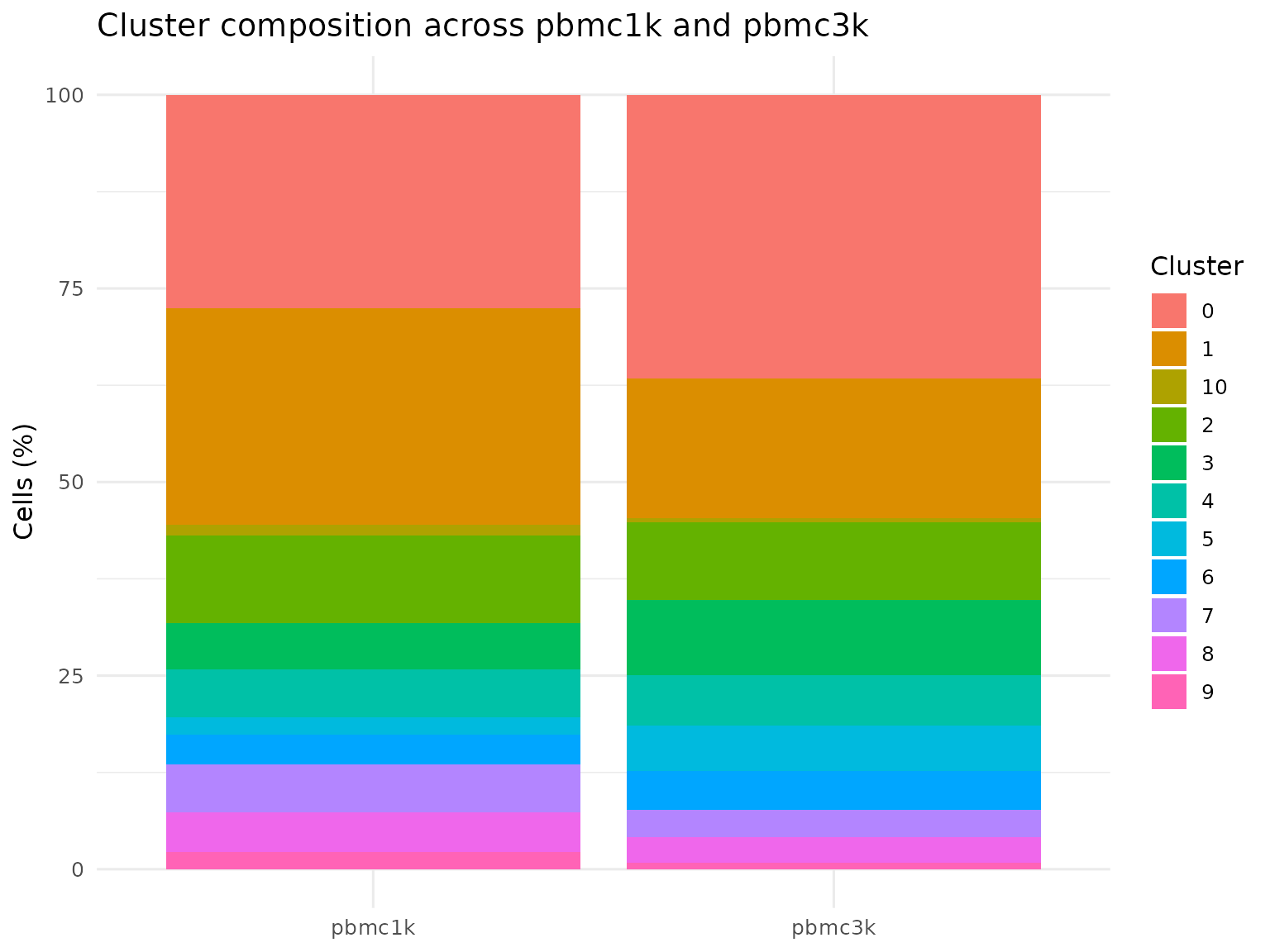
Integration quality summary with LISI
knitr::kable(lisi_summary, digits = 3)| state | min | q1 | median | mean | q3 | max |
|---|---|---|---|---|---|---|
| after_integration | 1.002 | 1.212 | 1.491 | 1.517 | 1.837 | 2 |
| before_integration | 1.000 | 1.000 | 1.000 | 1.024 | 1.000 | 2 |
Higher LISI values indicate better local sample mixing. In this two-sample example the theoretical maximum is 2, so the post-Harmony distribution should shift upward relative to the unintegrated baseline.
Multi-metric integration assessment
knitr::kable(assessment_summary, digits = 3)| metric | category | score | scaled_score | n_cells | source | note |
|---|---|---|---|---|---|---|
| batch_silhouette | batch_removal | 0.096 | 0.904 | 3812 | harmony | Global batch silhouette |
| batch_lisi | batch_removal | 1.517 | 0.517 | 3812 | harmony | |
| cluster_connectivity | structure | 1.000 | 1.000 | 3812 | RNA_nn | |
| pcr_batch | batch_removal | 0.007 | 0.929 | 3812 | harmony vs pca |
sn_assess_integration() combines local sample mixing,
PCR batch reduction, graph connectivity, isolated-label preservation,
cluster batch entropy, cluster purity, and difficult-group diagnostics
into one summary object while reusing the stored neighbor graph when
possible.
knitr::kable(challenging_groups, digits = 3)| seurat_clusters | n_cells | fraction_cells | median_neighbor_purity | mean_neighbor_purity | graph_connectivity | mean_silhouette | separation_score | challenge_score | rare_group | challenging_group |
|---|---|---|---|---|---|---|---|---|---|---|
| 9 | 48 | 0.013 | 0.956 | 0.836 | 1 | -0.041 | 0.812 | 0.188 | TRUE | FALSE |
| 8 | 146 | 0.038 | 0.969 | 0.903 | 1 | 0.102 | 0.840 | 0.160 | FALSE | FALSE |
| 3 | 329 | 0.086 | 1.000 | 0.886 | 1 | 0.058 | 0.843 | 0.157 | FALSE | FALSE |
| 0 | 1293 | 0.339 | 1.000 | 0.977 | 1 | 0.196 | 0.866 | 0.134 | FALSE | FALSE |
| 4 | 244 | 0.064 | 1.000 | 0.952 | 1 | 0.223 | 0.870 | 0.130 | FALSE | FALSE |
| 2 | 395 | 0.104 | 1.000 | 0.967 | 1 | 0.281 | 0.880 | 0.120 | FALSE | FALSE |
| 6 | 177 | 0.046 | 1.000 | 0.907 | 1 | 0.305 | 0.884 | 0.116 | FALSE | FALSE |
| 7 | 165 | 0.043 | 1.000 | 0.939 | 1 | 0.313 | 0.886 | 0.114 | FALSE | FALSE |
| 5 | 184 | 0.048 | 1.000 | 0.962 | 1 | 0.376 | 0.896 | 0.104 | FALSE | FALSE |
| 1 | 801 | 0.210 | 1.000 | 0.987 | 1 | 0.378 | 0.896 | 0.104 | FALSE | FALSE |
| 10 | 30 | 0.008 | 1.000 | 0.995 | 1 | 0.738 | 0.956 | 0.044 | TRUE | FALSE |
The challenging_groups table is especially useful for
surfacing rare groups or poorly separated populations that may not stand
out as isolated UMAP islands.
knitr::kable(integration_assessment$per_group$isolated_label_score, digits = 3)The isolated-label summary makes it easier to spot small populations that stay biologically distinct even when they do not appear as a visually isolated UMAP island after integration.
Rare-aware feature selection
When small populations are a concern, sn_run_cluster()
can append rare-aware features to the main HVG set before PCA and
Harmony. In this article the integrated object was run with
rare_feature_method = "gini", and the resulting rare-cell
scores can be inspected directly:
knitr::kable(head(rare_detection[order(rare_detection$rare_score, decreasing = TRUE), ], 10), digits = 3)| cell_id | method | rare_score | rare_cell | |
|---|---|---|---|---|
| 640 | pbmc1k_GCCGTGAGTCAGTCCG-1 | gini | 79.314 | TRUE |
| 838 | pbmc1k_TACCGGGTCCTCGATC-1 | gini | 78.042 | TRUE |
| 1040 | pbmc1k_TGTAACGGTTGCGTAT-1 | gini | 71.848 | TRUE |
| 148 | pbmc1k_AGCCAGCGTAGTTAGA-1 | gini | 69.761 | TRUE |
| 674 | pbmc1k_GGATCTAGTGCCTGCA-1 | gini | 69.457 | TRUE |
| 1093 | pbmc1k_TTCCTAAGTGACGTCC-1 | gini | 63.962 | TRUE |
| 801 | pbmc1k_GTGTTCCGTAGTTCCA-1 | gini | 61.457 | TRUE |
| 32 | pbmc1k_AACGAAAAGGTTGGTG-1 | gini | 52.102 | TRUE |
| 1089 | pbmc1k_TTCCACGAGGAAGTGA-1 | gini | 47.752 | TRUE |
| 192 | pbmc1k_AGTCACATCTCCCATG-1 | gini | 47.373 | TRUE |
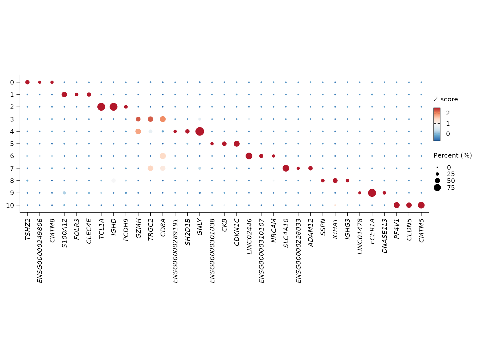
Marker genes from the integrated object
knitr::kable(marker_tbl, digits = 3)| cluster | gene | avg_log2FC | p_val_adj |
|---|---|---|---|
| 0 | TSHZ2 | 5.214 | 0 |
| 0 | ENSG00000249806 | 4.826 | 0 |
| 0 | CMTM8 | 3.704 | 0 |
| 1 | S100A12 | 8.653 | 0 |
| 1 | FOLR3 | 8.427 | 0 |
| 1 | CLEC4E | 7.854 | 0 |
| 2 | TCL1A | 8.067 | 0 |
| 2 | IGHD | 6.823 | 0 |
| 2 | PCDH9 | 6.358 | 0 |
| 3 | GZMH | 4.361 | 0 |
| 3 | TRGC2 | 4.120 | 0 |
| 3 | CD8A | 3.721 | 0 |
| 4 | ENSG00000289191 | 7.495 | 0 |
| 4 | SH2D1B | 7.266 | 0 |
| 4 | GNLY | 7.205 | 0 |
| 5 | ENSG00000301038 | 8.430 | 0 |
| 5 | CKB | 7.015 | 0 |
| 5 | CDKN1C | 6.909 | 0 |
| 6 | LINC02446 | 5.616 | 0 |
| 6 | ENSG00000310107 | 4.854 | 0 |
| 6 | NRCAM | 4.647 | 0 |
| 7 | SLC4A10 | 7.660 | 0 |
| 7 | ENSG00000228033 | 7.646 | 0 |
| 7 | ADAM12 | 6.413 | 0 |
| 8 | SSPN | 8.885 | 0 |
| 8 | IGHA1 | 8.245 | 0 |
| 8 | IGHG3 | 7.907 | 0 |
| 9 | LINC01478 | 10.605 | 0 |
| 9 | FCER1A | 8.531 | 0 |
| 9 | DNASE1L3 | 8.426 | 0 |
| 10 | PF4V1 | 15.175 | 0 |
| 10 | CLDN5 | 13.563 | 0 |
| 10 | CMTM5 | 13.046 | 0 |
sn_plot_dot(
  x = pbmc_integrated,
  features = "top_markers",
  de_name = "cluster_markers",
  n = 3
)
Functional enrichment of marker genes
The table below shows the first non-empty GO Biological Process GSEA result found among the cluster marker sets. In this run, enrichment was computed from cluster 0.
knitr::kable(enrichment_tbl, digits = 4)| ID | Description | NES | p.adjust | |
|---|---|---|---|---|
| GO:0002250 | GO:0002250 | adaptive immune response | 2.2222 | 0 |
| GO:0042110 | GO:0042110 | T cell activation | 2.1480 | 0 |
| GO:0046649 | GO:0046649 | lymphocyte activation | 1.9937 | 0 |
| GO:0001775 | GO:0001775 | cell activation | 1.9338 | 0 |
| GO:0045321 | GO:0045321 | leukocyte activation | 1.9244 | 0 |
| GO:0006955 | GO:0006955 | immune response | 1.8855 | 0 |
| GO:1903131 | GO:1903131 | mononuclear cell differentiation | 2.0001 | 0 |
| GO:0002684 | GO:0002684 | positive regulation of immune system process | 1.9479 | 0 |
| GO:0002682 | GO:0002682 | regulation of immune system process | 1.8416 | 0 |
| GO:0002768 | GO:0002768 | immune response-regulating cell surface receptor signaling pathway | 2.1336 | 0 |
sessioninfo::session_info()
#> ─ Session info ───────────────────────────────────────────────────────────────
#>  setting  value
#>  version  R version 4.5.3 (2026-03-11)
#>  os       Ubuntu 24.04.3 LTS
#>  system   x86_64, linux-gnu
#>  ui       X11
#>  language en
#>  collate  C.UTF-8
#>  ctype    C.UTF-8
#>  tz       UTC
#>  date     2026-03-26
#>  pandoc   3.1.11 @ /opt/hostedtoolcache/pandoc/3.1.11/x64/ (via rmarkdown)
#>  quarto   NA
#>
#> ─ Packages ───────────────────────────────────────────────────────────────────
#>  package           * version  date (UTC) lib source
#>  abind               1.4-8    2024-09-12 [1] CRAN (R 4.5.3)
#>  AnnotationDbi       1.72.0   2025-10-29 [1] Bioconduc~
#>  ape                 5.8-1    2024-12-16 [1] CRAN (R 4.5.3)
#>  aplot               0.2.9    2025-09-12 [1] CRAN (R 4.5.3)
#>  Biobase             2.70.0   2025-10-29 [1] Bioconduc~
#>  BiocGenerics        0.56.0   2025-10-29 [1] Bioconduc~
#>  BiocParallel        1.44.0   2025-10-29 [1] Bioconduc~
#>  Biostrings          2.78.0   2025-10-29 [1] Bioconduc~
#>  bit                 4.6.0    2025-03-06 [1] CRAN (R 4.5.3)
#>  bit64               4.6.0-1  2025-01-16 [1] CRAN (R 4.5.3)
#>  blob                1.3.0    2026-01-14 [1] CRAN (R 4.5.3)
#>  bslib               0.10.0   2026-01-26 [1] CRAN (R 4.5.3)
#>  cachem              1.1.0    2024-05-16 [1] CRAN (R 4.5.3)
#>  catplot             0.1.0    2026-03-19 [1] Github (catplot/catplot@0fc2344)
#>  cli                 3.6.5    2025-04-23 [1] CRAN (R 4.5.3)
#>  cluster             2.1.8.2  2026-02-05 [3] CRAN (R 4.5.3)
#>  clusterProfiler     4.18.4   2025-12-15 [1] any (@4.18.4)
#>  codetools           0.2-20   2024-03-31 [3] CRAN (R 4.5.3)
#>  cowplot             1.2.0    2025-07-07 [1] CRAN (R 4.5.3)
#>  crayon              1.5.3    2024-06-20 [1] CRAN (R 4.5.3)
#>  curl                7.0.0    2025-08-19 [1] CRAN (R 4.5.3)
#>  data.table          1.18.2.1 2026-01-27 [1] CRAN (R 4.5.3)
#>  DBI                 1.3.0    2026-02-25 [1] CRAN (R 4.5.3)
#>  deldir              2.0-4    2024-02-28 [1] CRAN (R 4.5.3)
#>  desc                1.4.3    2023-12-10 [1] CRAN (R 4.5.3)
#>  digest              0.6.39   2025-11-19 [1] CRAN (R 4.5.3)
#>  DOSE                4.4.0    2025-10-29 [1] Bioconduc~
#>  dotCall64           1.2      2024-10-04 [1] CRAN (R 4.5.3)
#>  dplyr             * 1.2.0    2026-02-03 [1] CRAN (R 4.5.3)
#>  enrichplot          1.30.5   2026-03-02 [1] Bioconduc~
#>  evaluate            1.0.5    2025-08-27 [1] CRAN (R 4.5.3)
#>  farver              2.1.2    2024-05-13 [1] CRAN (R 4.5.3)
#>  fastDummies         1.7.5    2025-01-20 [1] CRAN (R 4.5.3)
#>  fastmap             1.2.0    2024-05-15 [1] CRAN (R 4.5.3)
#>  fastmatch           1.1-8    2026-01-17 [1] CRAN (R 4.5.3)
#>  fgsea               1.36.2   2026-01-05 [1] Bioconduc~
#>  fitdistrplus        1.2-6    2026-01-24 [1] CRAN (R 4.5.3)
#>  fontBitstreamVera   0.1.1    2017-02-01 [1] CRAN (R 4.5.3)
#>  fontLiberation      0.1.0    2016-10-15 [1] CRAN (R 4.5.3)
#>  fontquiver          0.2.1    2017-02-01 [1] CRAN (R 4.5.3)
#>  fs                  2.0.1    2026-03-24 [1] CRAN (R 4.5.3)
#>  future            * 1.70.0   2026-03-14 [1] CRAN (R 4.5.3)
#>  future.apply        1.20.2   2026-02-20 [1] CRAN (R 4.5.3)
#>  gdtools             0.5.0    2026-02-09 [1] CRAN (R 4.5.3)
#>  generics            0.1.4    2025-05-09 [1] CRAN (R 4.5.3)
#>  ggforce             0.5.0    2025-06-18 [1] CRAN (R 4.5.3)
#>  ggfun               0.2.0    2025-07-15 [1] CRAN (R 4.5.3)
#>  ggiraph             0.9.6    2026-02-21 [1] CRAN (R 4.5.3)
#>  ggnewscale          0.5.2    2025-06-20 [1] CRAN (R 4.5.3)
#>  ggplot2           * 4.0.2    2026-02-03 [1] CRAN (R 4.5.3)
#>  ggplotify           0.1.3    2025-09-20 [1] CRAN (R 4.5.3)
#>  ggrepel             0.9.8    2026-03-17 [1] CRAN (R 4.5.3)
#>  ggridges            0.5.7    2025-08-27 [1] CRAN (R 4.5.3)
#>  ggtangle            0.1.1    2026-01-16 [1] CRAN (R 4.5.3)
#>  ggtree              4.0.5    2026-03-17 [1] Bioconduc~
#>  globals             0.19.1   2026-03-13 [1] CRAN (R 4.5.3)
#>  glue                1.8.0    2024-09-30 [1] CRAN (R 4.5.3)
#>  GO.db               3.22.0   2026-03-19 [1] Bioconductor
#>  goftest             1.2-3    2021-10-07 [1] CRAN (R 4.5.3)
#>  GOSemSim            2.36.0   2025-10-29 [1] Bioconduc~
#>  gridExtra           2.3      2017-09-09 [1] CRAN (R 4.5.3)
#>  gridGraphics        0.5-1    2020-12-13 [1] CRAN (R 4.5.3)
#>  gson                0.1.0    2023-03-07 [1] CRAN (R 4.5.3)
#>  gtable              0.3.6    2024-10-25 [1] CRAN (R 4.5.3)
#>  harmony             2.0.0    2026-03-24 [1] Github (immunogenomics/harmony@3617c00)
#>  hdf5r               1.3.12   2025-01-20 [1] any (@1.3.12)
#>  HGNChelper          0.8.15   2024-11-16 [1] any (@0.8.15)
#>  htmltools           0.5.9    2025-12-04 [1] CRAN (R 4.5.3)
#>  htmlwidgets         1.6.4    2023-12-06 [1] CRAN (R 4.5.3)
#>  httpuv              1.6.17   2026-03-18 [1] CRAN (R 4.5.3)
#>  httr                1.4.8    2026-02-13 [1] CRAN (R 4.5.3)
#>  ica                 1.0-3    2022-07-08 [1] CRAN (R 4.5.3)
#>  igraph              2.2.2    2026-02-12 [1] CRAN (R 4.5.3)
#>  IRanges             2.44.0   2025-10-29 [1] Bioconduc~
#>  irlba               2.3.7    2026-01-30 [1] CRAN (R 4.5.3)
#>  jquerylib           0.1.4    2021-04-26 [1] CRAN (R 4.5.3)
#>  jsonlite            2.0.0    2025-03-27 [1] CRAN (R 4.5.3)
#>  KEGGREST            1.50.0   2025-10-29 [1] Bioconduc~
#>  KernSmooth          2.23-26  2025-01-01 [3] CRAN (R 4.5.3)
#>  knitr             * 1.51     2025-12-20 [1] CRAN (R 4.5.3)
#>  labeling            0.4.3    2023-08-29 [1] CRAN (R 4.5.3)
#>  later               1.4.8    2026-03-05 [1] CRAN (R 4.5.3)
#>  lattice             0.22-9   2026-02-09 [3] CRAN (R 4.5.3)
#>  lazyeval            0.2.2    2019-03-15 [1] CRAN (R 4.5.3)
#>  lifecycle           1.0.5    2026-01-08 [1] CRAN (R 4.5.3)
#>  limma               3.66.0   2025-10-29 [1] Bioconduc~
#>  lisi                1.0      2026-03-19 [1] Github (immunogenomics/lisi@a917556)
#>  listenv             0.10.1   2026-03-10 [1] CRAN (R 4.5.3)
#>  lmtest              0.9-40   2022-03-21 [1] CRAN (R 4.5.3)
#>  logger              0.4.1    2025-09-11 [1] CRAN (R 4.5.3)
#>  magrittr            2.0.4    2025-09-12 [1] CRAN (R 4.5.3)
#>  MASS                7.3-65   2025-02-28 [3] CRAN (R 4.5.3)
#>  Matrix              1.7-4    2025-08-28 [3] CRAN (R 4.5.3)
#>  matrixStats         1.5.0    2025-01-07 [1] CRAN (R 4.5.3)
#>  memoise             2.0.1    2021-11-26 [1] CRAN (R 4.5.3)
#>  mime                0.13     2025-03-17 [1] CRAN (R 4.5.3)
#>  miniUI              0.1.2    2025-04-17 [1] CRAN (R 4.5.3)
#>  nlme                3.1-168  2025-03-31 [3] CRAN (R 4.5.3)
#>  org.Hs.eg.db        3.22.0   2026-03-19 [1] bioc (@3.22.0)
#>  otel                0.2.0    2025-08-29 [1] CRAN (R 4.5.3)
#>  parallelly          1.46.1   2026-01-08 [1] CRAN (R 4.5.3)
#>  patchwork           1.3.2    2025-08-25 [1] CRAN (R 4.5.3)
#>  pbapply             1.7-4    2025-07-20 [1] CRAN (R 4.5.3)
#>  pillar              1.11.1   2025-09-17 [1] CRAN (R 4.5.3)
#>  pkgconfig           2.0.3    2019-09-22 [1] CRAN (R 4.5.3)
#>  pkgdown             2.2.0    2025-11-06 [1] any (@2.2.0)
#>  plotly              4.12.0   2026-01-24 [1] CRAN (R 4.5.3)
#>  plyr                1.8.9    2023-10-02 [1] CRAN (R 4.5.3)
#>  png                 0.1-9    2026-03-15 [1] CRAN (R 4.5.3)
#>  polyclip            1.10-7   2024-07-23 [1] CRAN (R 4.5.3)
#>  progressr           0.18.0   2025-11-06 [1] CRAN (R 4.5.3)
#>  promises            1.5.0    2025-11-01 [1] CRAN (R 4.5.3)
#>  purrr               1.2.1    2026-01-09 [1] CRAN (R 4.5.3)
#>  qvalue              2.42.0   2025-10-29 [1] Bioconduc~
#>  R.methodsS3         1.8.2    2022-06-13 [1] CRAN (R 4.5.3)
#>  R.oo                1.27.1   2025-05-02 [1] CRAN (R 4.5.3)
#>  R.utils             2.13.0   2025-02-24 [1] CRAN (R 4.5.3)
#>  R6                  2.6.1    2025-02-15 [1] CRAN (R 4.5.3)
#>  ragg                1.5.2    2026-03-23 [1] CRAN (R 4.5.3)
#>  RANN                2.6.2    2024-08-25 [1] CRAN (R 4.5.3)
#>  rappdirs            0.3.4    2026-01-17 [1] CRAN (R 4.5.3)
#>  RColorBrewer        1.1-3    2022-04-03 [1] CRAN (R 4.5.3)
#>  Rcpp                1.1.1    2026-01-10 [1] CRAN (R 4.5.3)
#>  RcppAnnoy           0.0.23   2026-01-12 [1] CRAN (R 4.5.3)
#>  RcppHNSW            0.6.0    2024-02-04 [1] CRAN (R 4.5.3)
#>  reshape2            1.4.5    2025-11-12 [1] CRAN (R 4.5.3)
#>  reticulate          1.45.0   2026-02-13 [1] CRAN (R 4.5.3)
#>  RhpcBLASctl         0.23-42  2023-02-11 [1] CRAN (R 4.5.3)
#>  rio                 1.2.4    2025-09-26 [1] any (@1.2.4)
#>  rlang               1.1.7    2026-01-09 [1] CRAN (R 4.5.3)
#>  rmarkdown           2.31     2026-03-26 [1] CRAN (R 4.5.3)
#>  ROCR                1.0-12   2026-01-23 [1] CRAN (R 4.5.3)
#>  RSpectra            0.16-2   2024-07-18 [1] CRAN (R 4.5.3)
#>  RSQLite             2.4.6    2026-02-06 [1] CRAN (R 4.5.3)
#>  Rtsne               0.17     2023-12-07 [1] CRAN (R 4.5.3)
#>  S4Vectors           0.48.0   2025-10-29 [1] Bioconduc~
#>  S7                  0.2.1    2025-11-14 [1] CRAN (R 4.5.3)
#>  sass                0.4.10   2025-04-11 [1] CRAN (R 4.5.3)
#>  scales              1.4.0    2025-04-24 [1] CRAN (R 4.5.3)
#>  scattermore         1.2      2023-06-12 [1] CRAN (R 4.5.3)
#>  scatterpie          0.2.6    2025-09-12 [1] CRAN (R 4.5.3)
#>  sctransform         0.4.3    2026-01-10 [1] CRAN (R 4.5.3)
#>  Seqinfo             1.0.0    2025-10-29 [1] Bioconduc~
#>  sessioninfo         1.2.3    2025-02-05 [1] any (@1.2.3)
#>  Seurat            * 5.4.0    2025-12-14 [1] any (@5.4.0)
#>  SeuratObject      * 5.3.0    2025-12-12 [1] CRAN (R 4.5.3)
#>  Shennong          * 0.1.2    2026-03-26 [1] local
#>  shiny               1.13.0   2026-02-20 [1] CRAN (R 4.5.3)
#>  sp                * 2.2-1    2026-02-13 [1] CRAN (R 4.5.3)
#>  spam                2.11-3   2026-01-08 [1] CRAN (R 4.5.3)
#>  spatstat.data       3.1-9    2025-10-18 [1] CRAN (R 4.5.3)
#>  spatstat.explore    3.8-0    2026-03-22 [1] CRAN (R 4.5.3)
#>  spatstat.geom       3.7-3    2026-03-23 [1] CRAN (R 4.5.3)
#>  spatstat.random     3.4-5    2026-03-22 [1] CRAN (R 4.5.3)
#>  spatstat.sparse     3.1-0    2024-06-21 [1] CRAN (R 4.5.3)
#>  spatstat.univar     3.1-7    2026-03-18 [1] CRAN (R 4.5.3)
#>  spatstat.utils      3.2-2    2026-03-10 [1] CRAN (R 4.5.3)
#>  splitstackshape     1.4.8.1  2026-03-21 [1] CRAN (R 4.5.3)
#>  statmod             1.5.1    2025-10-09 [1] CRAN (R 4.5.3)
#>  stringi             1.8.7    2025-03-27 [1] CRAN (R 4.5.3)
#>  stringr             1.6.0    2025-11-04 [1] CRAN (R 4.5.3)
#>  survival            3.8-6    2026-01-16 [3] CRAN (R 4.5.3)
#>  systemfonts         1.3.2    2026-03-05 [1] CRAN (R 4.5.3)
#>  tensor              1.5.1    2025-06-17 [1] CRAN (R 4.5.3)
#>  textshaping         1.0.5    2026-03-06 [1] CRAN (R 4.5.3)
#>  tibble              3.3.1    2026-01-11 [1] CRAN (R 4.5.3)
#>  tictoc              1.2.1    2024-03-18 [1] CRAN (R 4.5.3)
#>  tidydr              0.0.6    2025-07-25 [1] CRAN (R 4.5.3)
#>  tidyr               1.3.2    2025-12-19 [1] CRAN (R 4.5.3)
#>  tidyselect          1.2.1    2024-03-11 [1] CRAN (R 4.5.3)
#>  tidytree            0.4.7    2026-01-08 [1] CRAN (R 4.5.3)
#>  treeio              1.34.0   2025-10-30 [1] Bioconduc~
#>  tweenr              2.0.3    2024-02-26 [1] CRAN (R 4.5.3)
#>  utf8                1.2.6    2025-06-08 [1] CRAN (R 4.5.3)
#>  uwot                0.2.4    2025-11-10 [1] CRAN (R 4.5.3)
#>  vctrs               0.7.2    2026-03-21 [1] CRAN (R 4.5.3)
#>  viridisLite         0.4.3    2026-02-04 [1] CRAN (R 4.5.3)
#>  withr               3.0.2    2024-10-28 [1] CRAN (R 4.5.3)
#>  xfun                0.57     2026-03-20 [1] CRAN (R 4.5.3)
#>  xtable              1.8-8    2026-02-22 [1] CRAN (R 4.5.3)
#>  XVector             0.50.0   2025-10-29 [1] Bioconduc~
#>  yaml                2.3.12   2025-12-10 [1] CRAN (R 4.5.3)
#>  yulab.utils         0.2.4    2026-02-02 [1] CRAN (R 4.5.3)
#>  zoo                 1.8-15   2025-12-15 [1] CRAN (R 4.5.3)
#>
#>  [1] /home/runner/work/_temp/Library
#>  [2] /opt/R/4.5.3/lib/R/site-library
#>  [3] /opt/R/4.5.3/lib/R/library
#>  * ── Packages attached to the search path.
#>
#> ──────────────────────────────────────────────────────────────────────────────