Annotation, markers, and pathways workflow

This article covers the main biological-interpretation stage after clustering:

inspect bundled signatures
score marker structure with differential expression
visualize top markers
run ORA or GSEA with sn_enrich()
optionally bring in reference-based annotation with sn_run_celltypist()

library(Shennong)
library(dplyr)
library(knitr)
library(Seurat)

if (!exists("pbmc_small", inherits = FALSE)) {
  try(data("pbmc_small", package = "Shennong", envir = environment()), silent = TRUE)
}
if (!exists("pbmc_small", inherits = FALSE) && file.exists(file.path("data", "pbmc_small.rda"))) {
  load(file.path("data", "pbmc_small.rda"))
}

1. Start from bundled signatures

Bundled signatures provide a stable set of marker programs and technical gene sets for filtering, scoring, or interpretation.

knitr::kable(head(signature_tbl[, c("path", "n_genes")], 8))

path	n_genes
Blocklists/Pseudogenes	12600
Blocklists/Non-coding	7783
Programs/HeatShock	97
Programs/cellCycle.G1S	42
Programs/cellCycle.G2M	52
Programs/IFN	107
Programs/Tcell.cytotoxicity	3
Programs/Tcell.exhaustion	5

length(stress_genes)
#> [1] 134

2. Find marker genes

Cluster markers are usually the first evidence layer for annotation.

knitr::kable(marker_tbl)

p_val	avg_log2FC	pct.1	pct.2	p_val_adj	cluster	gene
8.9e-06	5.159201	0.330	0.101	0.4901319	0	NKG7
7.0e-07	5.143783	0.352	0.092	0.0407973	0	CCL5
1.0e-07	4.070451	0.330	0.046	0.0039324	0	GZMA
0.0e+00	9.635408	0.533	0.000	0.0000000	1	LRMDA
0.0e+00	9.603413	0.444	0.000	0.0000000	1	S100A12
0.0e+00	9.137996	0.422	0.000	0.0000000	1	IL1B
0.0e+00	6.317317	0.257	0.000	0.0000017	2	CA6
0.0e+00	6.152965	0.286	0.000	0.0000001	2	TRPC1
0.0e+00	6.144032	0.314	0.000	0.0000000	2	OPRM1
0.0e+00	11.461813	0.379	0.000	0.0000000	3	IGLC2
0.0e+00	10.040121	0.690	0.000	0.0000000	3	IGHD
0.0e+00	9.743428	0.586	0.000	0.0000000	3	TCL1A

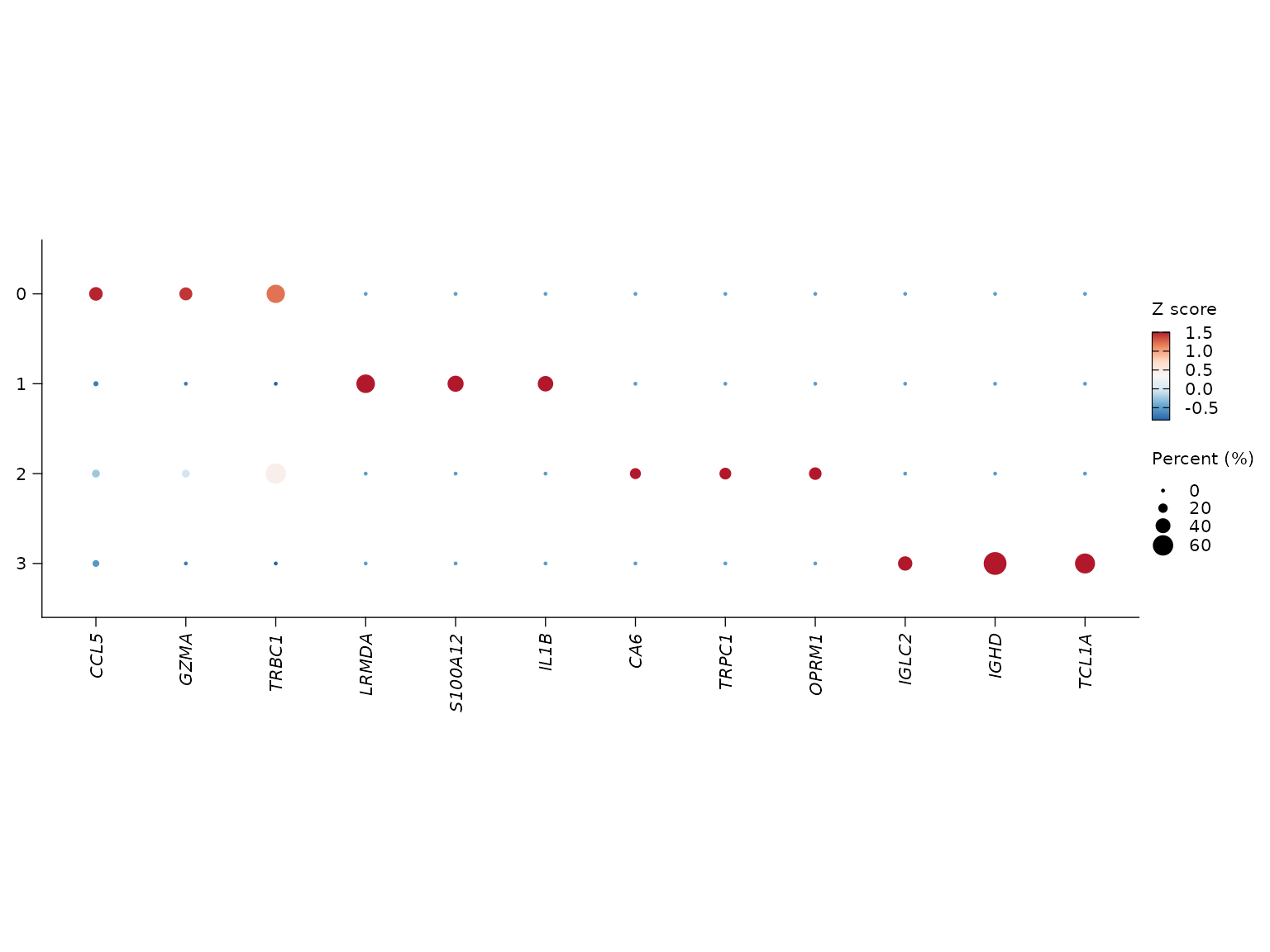
3. Visualize top markers

sn_plot_dot() can reuse the stored DE result directly, which avoids manual gene selection in routine cluster review.

sn_plot_dot(
  pbmc_clustered,
  features = "top_markers",
  de_name = "cluster_markers",
  n = 3
)

4. Run pathway analysis

sn_enrich() now supports grouped ORA and ranked GSEA through the same gene_clusters formula interface. It can also query multiple databases in one call.

if (!is.null(stored_pathways)) {
  knitr::kable(stored_pathways, digits = 4)
}

Grouped ORA uses a categorical right-hand side:

ora_result <- sn_enrich(
  x = pbmc_clustered,
  source_de_name = "cluster_markers",
  gene_clusters = gene ~ cluster,
  database = c("H", "C2:CP:REACTOME"),
  species = "human"
)

Ranked GSEA uses a numeric right-hand side:

gsea_result <- sn_enrich(
  marker_table,
  gene_clusters = gene ~ avg_log2FC,
  database = "GOBP",
  species = "human"
)

5. Optional reference-based annotation

If CellTypist is configured in the local environment, Shennong can add reference labels to the Seurat object:

pbmc_annotated <- sn_run_celltypist(
  pbmc_clustered,
  model = "Immune_All_Low.pkl"
)

That annotation can then be reused as the label input for downstream integration metrics or cluster summaries.

Songqi Duan

1. Start from bundled signatures

2. Find marker genes

3. Visualize top markers

4. Run pathway analysis

5. Optional reference-based annotation